How To Get Residual Plot On Ti-84

Alright, buckle up buttercups! You're about to become a residual plot rockstar, all thanks to your trusty TI-84 calculator! It's easier than ordering pizza, I promise!

First Things First: Data Entry!

Grab your data – sales figures versus advertising spend, maybe? Anything goes! Now, fire up your TI-84 and hit that glorious "STAT" button. It's usually hanging out somewhere near the directional arrows.

A menu pops up, right? Use those arrows to scoot over to "EDIT" and then select "1: Edit..." You're basically telling your calculator, "Hey, I've got data to share!".

See those lovely lists, L1, L2, L3...? L1 is your x-values (independent variable), and L2 is where your y-values (dependent variable) will reside. Type in your numbers, hitting "ENTER" after each one. Think of it as feeding your calculator a delicious data smoothie!

Time for Regression!

Okay, with data loaded, let's get regressing! Hit that "STAT" button again. Arrow over to "CALC" this time. We're cooking up a regression equation, baby!

You've got choices galore, but let's keep it simple. Choose "4: LinReg(ax+b)". This means we are doing a linear regression. Hit "ENTER" and the calculator will prompt you for the x-list and the y-list.

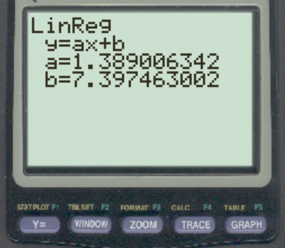
If you've stuck to L1 and L2, you can just hit "ENTER" a bunch of times. Otherwise, you'll need to tell the calculator which lists you used. Use the 2nd button with the number "1" or "2" to access L1 or L2. Now press "ENTER" until you see the glorious regression equation: y = ax + b, where *a* is the slope and *b* is the y-intercept.

Storing the Regression Equation

Now, this is a crucial step! We need to store that equation. Go back to the "STAT" -> "CALC" -> "4: LinReg(ax+b)" menu. Before you hit "ENTER", add a little magic!.

Tell the calculator where to store this equation. Hit "VARS," then "Y-VARS," then "1: Function," and finally "1: Y1". You're basically saying, "Hey calculator, shove this equation into Y1 for safekeeping!".

Now the line should look like: LinReg(ax+b) Y1. Press "ENTER." This command tells the calculator to calculate the linear regression and then store the resulting equation in Y1!

Generating the Residual List

Ready to create the magical residual list? This is where the fun REALLY begins! Hit "STAT" again, and then "EDIT." We're going to add a new list.

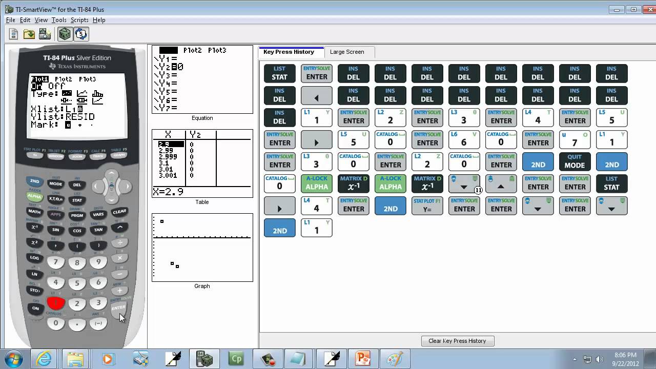
Arrow over to the heading of L3, and then press "ENTER." This will bring the cursor to the bottom of the list, with a blinking cursor at the bottom of L3. Now, let's tell the calculator what to put in list 3.

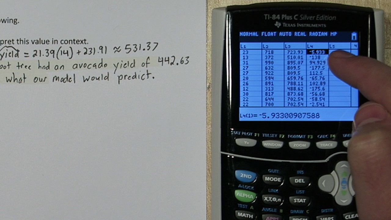
Type in: L2 - VARS -> Y-VARS -> 1: Function -> 1: Y1. This is how you get residuals on TI 84 calculator. What you are doing is subtracting the predicted values (Y1) from the actual values (L2). Once complete, press ENTER.

The calculator will automatically populate list L3 with the residuals. Prepare to be amazed!

Plotting Those Residuals!

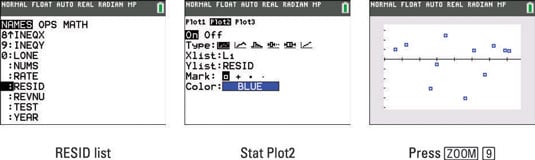
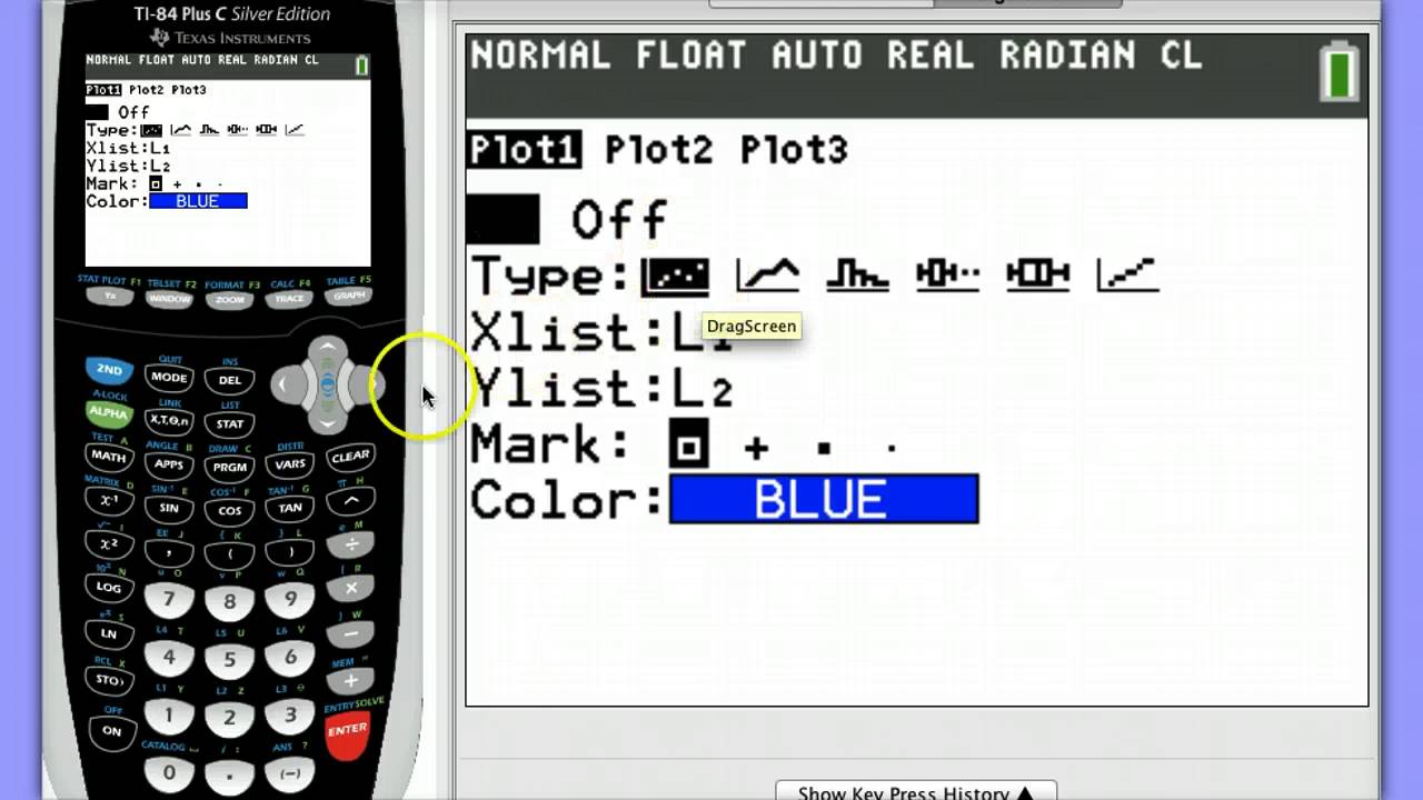
Almost there, champion! Now for the grand finale: plotting! Press 2nd and then "Y=" (the STAT PLOT button). This will take you to the Stat Plot menu. Make sure that Plot 1 is turned ON. Select Plot 1.

Turn the plot "On". Then, for "Type," select the scatter plot (the one with the little dots). It should be the first option.

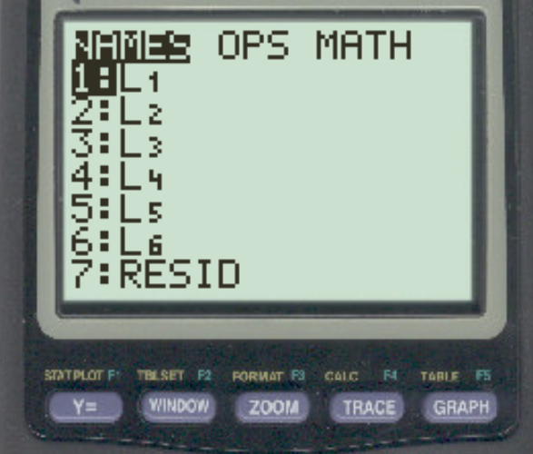
For "Xlist," select L1 (or whatever list contains your x-values). For "Ylist," select L3 (your awesome residual list!).

Finally, hit "ZOOM" and then "9: ZoomStat". This will magically adjust the window to perfectly display your residual plot! Voila! Bask in the glory of your residual plot. Analyze it, marvel at it, and feel the sweet, sweet satisfaction of data mastery!

If your residuals are randomly scattered, congratulations, my friend! You've got a pretty good linear model. If they form a pattern, well, Houston, we might have a nonlinearity problem. But that's a story for another time!