Sum Time In Excel Over 24 Hours

Excel users are facing a persistent hurdle: accurately summing time values exceeding 24 hours. Frustration is mounting as standard formulas fail to deliver correct totals for shifts, projects, and other time-tracking scenarios.

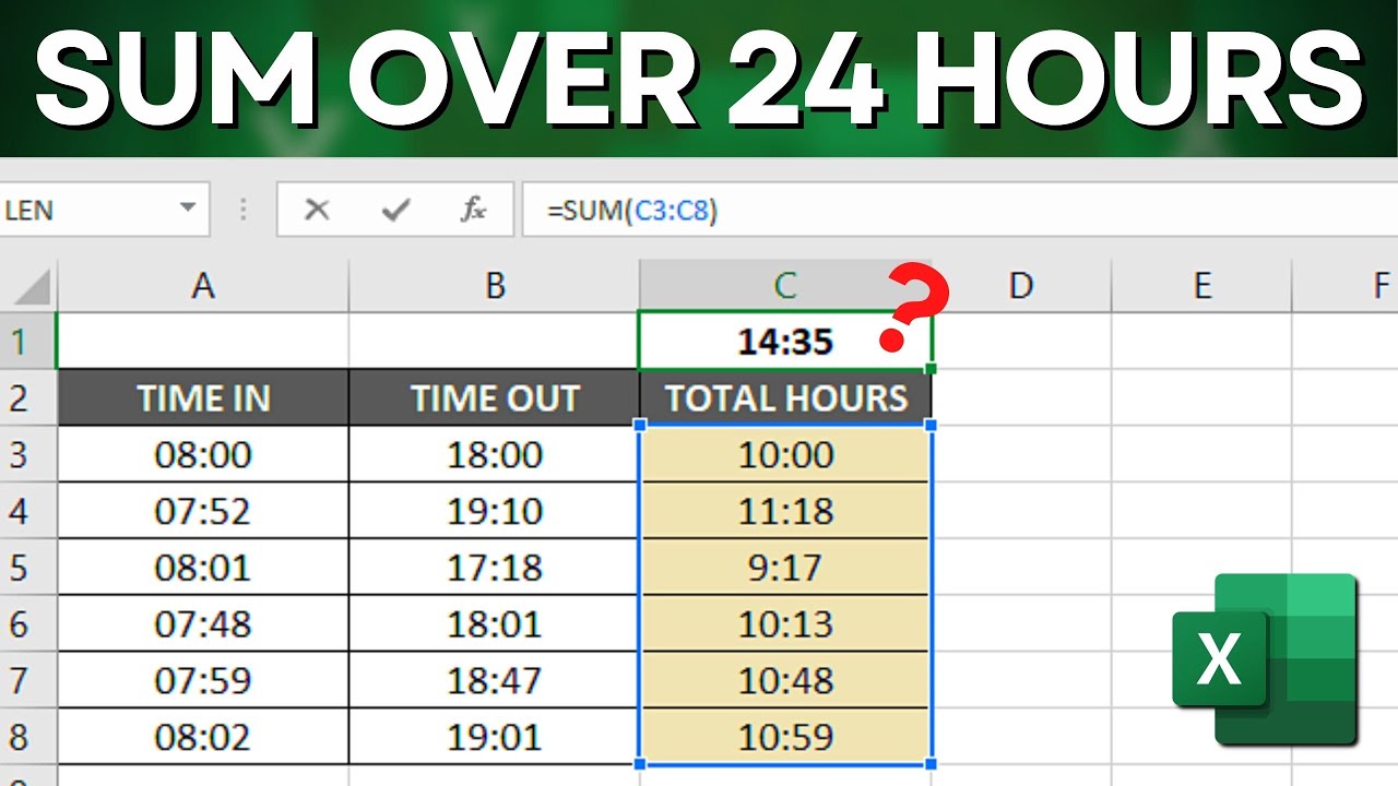
The issue stems from Excel's default handling of time values, which resets to zero after reaching 24 hours. This article breaks down the problem and provides immediate, actionable solutions to overcome this limitation.

The Problem: Excel's Time Format

Excel stores time as a fraction of a 24-hour day. For instance, "6:00 AM" is represented as 0.25 (6/24). The issue arises when the sum of these fractions exceeds 1, which Excel interprets as a new day, effectively resetting the time portion.

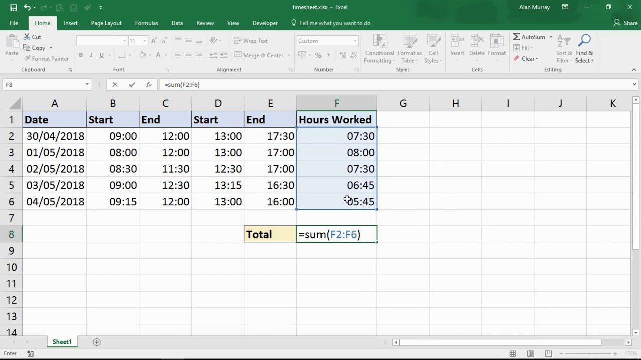
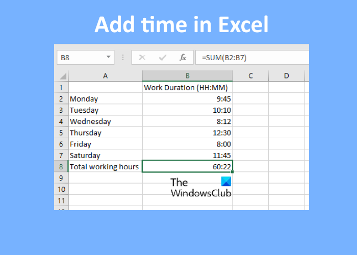
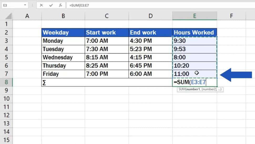
Users typically input time as "hours:minutes" (e.g., 8:30). Standard SUM functions then treat these entries as fractions, leading to incorrect totals.

The Culprit: Formatting Limitations

The root cause is the default formatting applied to cells containing time values. This formatting only displays time within a 24-hour cycle.

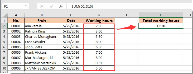
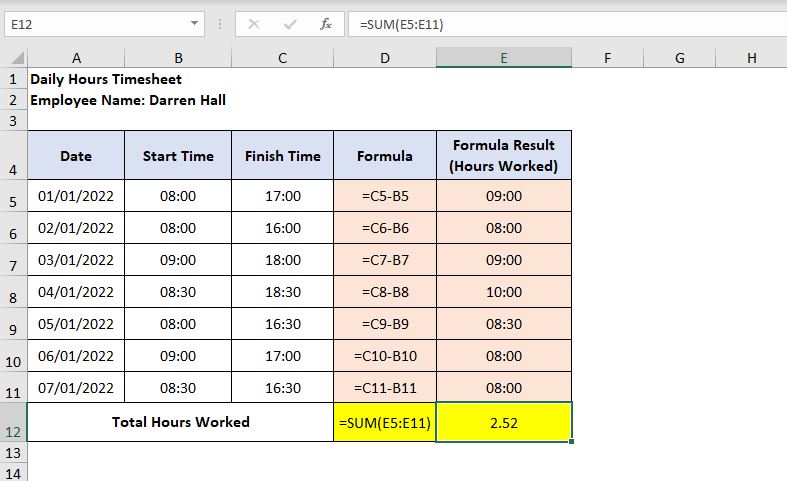
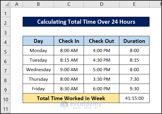
Without proper formatting adjustments, time totals exceeding 24 hours will "wrap around", showing only the remainder after a full day has passed. For example, a total of 30 hours might display as 6:00 (30 - 24 = 6).

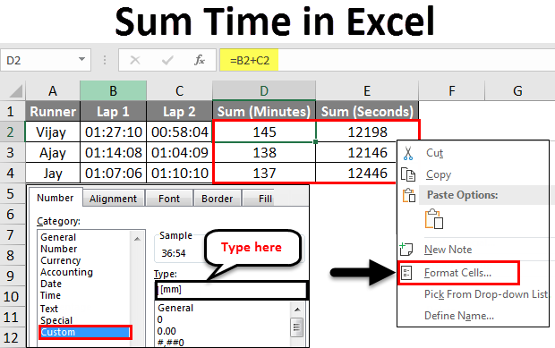
Solution 1: The Custom Format

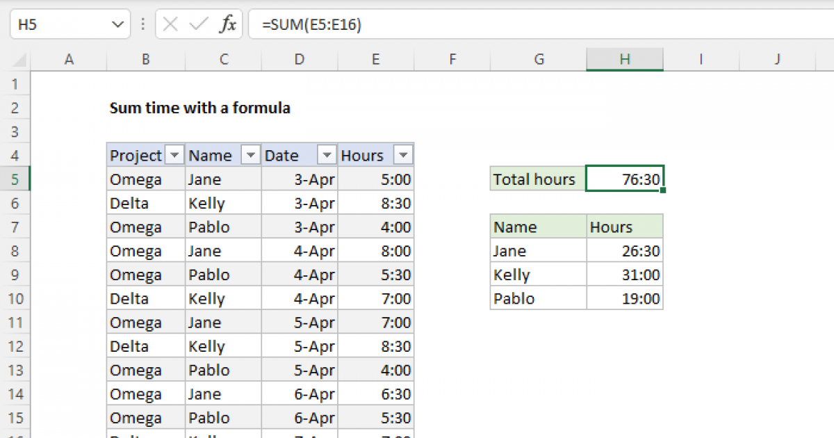
The most common and direct solution is to apply a custom format to the cell containing the summed time. This format instructs Excel to display the total number of hours, regardless of whether it exceeds 24.

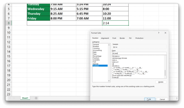
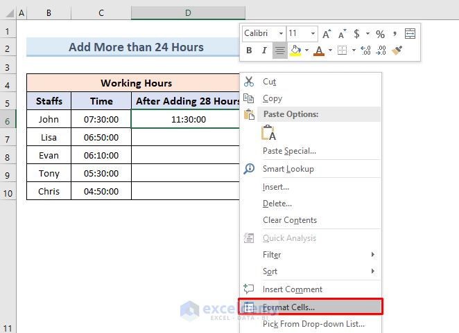
To apply the custom format: Right-click on the cell containing the time total. Select "Format Cells" then go to the "Number" tab. Choose "Custom" from the category list.

In the "Type" field, enter [h]:mm or [hh]:mm. The brackets around the "h" instruct Excel to display the total elapsed hours. Click "OK" to apply the format.

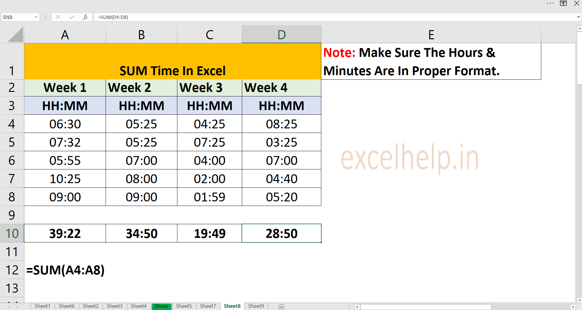
This custom format will now correctly display totals like 30:30 or 48:00, accurately reflecting the total time.

Solution 2: Using the TEXT Function

Another method involves using the TEXT function to format the time as text. This is particularly useful when you need to combine the time value with other text strings.

The syntax is: =TEXT(cell_containing_time, "[h]:mm"). Replace cell_containing_time with the actual cell reference (e.g., A1). This formula converts the time value into a text string formatted to display total hours and minutes.

For instance, =TEXT(A1, "[h]:mm")&" hours" would display "30:30 hours" if cell A1 contains a time value representing 30 hours and 30 minutes.

Solution 3: For More Complex Calculations

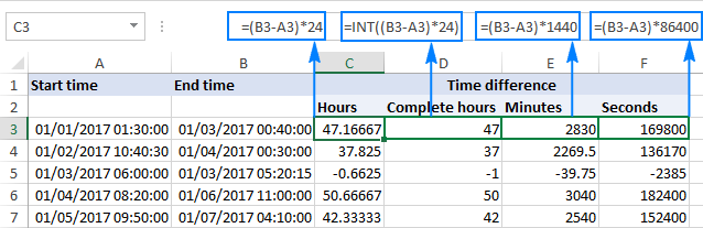
When time calculations involve days, hours, and minutes, a more robust formula may be necessary. One approach involves separating the day, hour, and minute components.

First, calculate the total hours by multiplying the day portion by 24 and adding it to the hour portion: =(INT(A1)*24)+HOUR(A1). Next, use the MINUTE function to extract the minutes: MINUTE(A1). Combine them to get the total time in hours and minutes.

However, this only gives you a numeric value. You might then want to present it in a user-friendly format using TEXT if presentation matters greatly.

Testing and Verification

After applying any solution, rigorously test the results to ensure accuracy. Use known time values and manually verify the calculated totals. Pay close attention to cases involving multiple days or partial days.

Double-check the cell formatting to confirm the custom format is correctly applied. Verify that formulas are referencing the correct cells and that there are no errors in the formula syntax.

Next Steps

Users encountering persistent issues should consult Microsoft's official Excel documentation or online forums. Consider sharing examples of the problematic data and the formulas being used.

Microsoft is actively working on enhancing Excel's time handling capabilities. Keep your Excel version up-to-date to benefit from potential improvements and bug fixes. Monitoring updates related to time and date formatting is advised.